Foundations of Digital Image Processing
January 15, 2026
Exploring mathematical discretization, statistical noise filtering, domain transformations, and production pipelines for facial recognition and liveness detection.
1. Statistical and Mathematical Foundations
Before diving into advanced computer vision models, understanding how physical light is translated into digital data is essential. This section covers the fundamental mathematics of discretization, statistical noise modeling, and transformation domains that form the bedrock of digital image manipulation.
1.1 Continuous vs. Discrete Functions
Conceptually, an ideal image is modeled as a continuous intensity function of two variables, $f(x,y)$. Here, $x$ and $y$ represent continuous spatial coordinates on the image plane, and $f(x,y)$ reflects the light intensity or grayscale level at that point. This formulation mirrors physical reality, where reflected light and sensor capture are continuous in both space and amplitude.
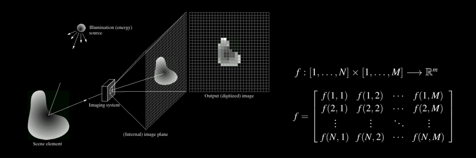
Because digital hardware cannot directly store continuous signals, the image must undergo discretization through two core steps: sampling and quantization.
- Sampling: Discretizes the spatial coordinates, mapping the continuous plane into a finite 2D grid. This transforms $f(x,y)$ into a discrete matrix $f[m, n]$, where $m$ and $n$ denote pixel indices. Higher sampling density yields finer spatial resolution.
- Quantization: Discretizes the intensity values. The continuous amplitude at each sample point maps to a discrete integer level (such as 0–255 for standard 8-bit depth). This step introduces quantization error, as distinct continuous values collapse into identical discrete bins.
Failing to sample at an adequate rate introduces aliasing artifacts like moiré patterns, while coarse quantization causes false contouring and banding across smooth gradients.
1.2 Probability and Statistics in Image Processing
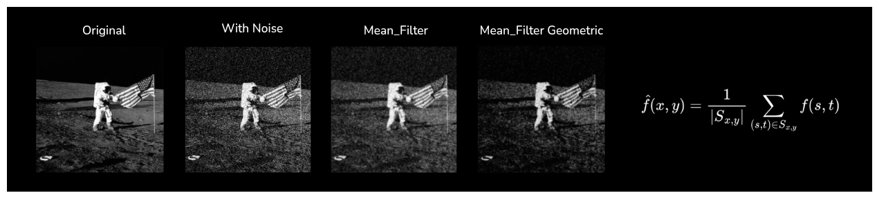
Images frequently pick up stochastic noise from sensor heat, poor lighting, or transmission interference. An observed noisy image $g[m,n]$ is commonly modeled by adding a random noise component $\eta[m,n]$ to the ideal image $f[m,n]$. Consequently, $g[m,n] = f[m,n] + \eta[m,n]$.
Filtering strategies directly depend on the statistical distribution of the noise:
- Gaussian Noise: Typically caused by thermal sensor fluctuations and governed by a normal distribution. The Mean Filter leverages statistical expectation by averaging local pixel neighborhoods to suppress random variance, though it softens sharp edges in the process.
- Salt-and-Pepper Noise: Manifests as extreme, impulsive black and white pixel spikes. The Median Filter, an order-statistic method, effectively eliminates these outliers without blurring adjacent structures by selecting the neighborhood median.
- Advanced Statistical Filters: Solutions like the Wiener Filter rely on second-order statistics (mean and variance) to minimize the Mean Square Error (MSE) between the estimated and original image, providing an optimal baseline for stationary Gaussian noise.
1.3 Mathematical Transformations and Domain Selection
Transforms allow us to analyze and manipulate images outside the traditional spatial coordinate system. The Fourier Transform maps spatial representations (intensity vs. coordinate) into the frequency domain (intensity vs. rate of change).
- Low-frequency components represent gradual intensity changes, corresponding to homogenous surfaces and global illumination.
- High-frequency components capture rapid spatial changes, such as sharp edges, fine textures, and high-frequency noise.
Selecting between domains depends entirely on the operational objective:
- Frequency Domain: Ideal for isolating and stripping out periodic noise patterns or targeted interference using low-pass, high-pass, or notch filters, which is computationally cleaner than extensive spatial convolutions.
- Spatial Domain: Well-suited for localized operations, including direct derivative-based sharpening kernels and local neighborhood smoothing.
2. Image Processing AI-Based Application
Translating theoretical image processing into practical systems requires integrating core transformations with modern machine learning architectures. Here, we examine the complete lifecycle of a facial recognition and liveness detection pipeline, from initial data capture to scalable production deployment.
2.1 Real-World Case Study: Facial Recognition Attendance System
In an automated attendance system, the computer vision pipeline moves through several sequential stages:
- Acquisition: Raw facial frames are captured from stationary cameras or mobile sensors, which inherently contain lighting shifts, pose variance, and sensor noise.
- Pre-processing: Applies standard image processing routines—resizing, intensity normalization, color conversions (e.g., RGB to grayscale), and denoising—to ensure consistent input formats for downstream models.
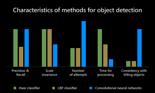
- Face Detection: Identifies and isolates facial boundaries using classical feature classifiers (such as Haar Cascades) or deep learning detectors (CNNs), generating localized bounding boxes.
- Feature Extraction: A deep CNN maps the isolated face crop into a compact, high-dimensional numerical embedding that uniquely encodes facial geometry rather than raw pixel intensities.
- Classification / Matching: The generated embedding is compared against indexed identities in a database using similarity metrics (such as cosine similarity) or classifiers (e.g., SVM, KNN). If the metric exceeds a confidence threshold, the attendance record is logged.
2.2 Simulation and Multi-Platform Development
Pipelines are initially prototyped and validated within frameworks like PyTorch or TensorFlow using benchmark datasets. Once accuracy targets are met, the model is exposed as a cloud/backend API service to serve mobile, web, and edge clients.
- Architecture: Decoupling compute-heavy image inference from application business logic via a microservices setup keeps the infrastructure maintainable and portable.
- UI/UX Asynchrony: Image capture and payload uploads run asynchronously to keep client interfaces responsive during heavy inference tasks.
- Database Strategy: A standard relational database handles administrative profiles, logs, and timestamps, while a dedicated vector database manages high-dimensional embeddings for rapid vector similarity lookups.
2.3 Evaluation and Industrial Scalability
Production systems must balance accuracy and operational speed. Robustness against uneven lighting, partial occlusions, and off-axis poses must be verified alongside low end-to-end latency to avoid bottlenecks. Techniques like model quantization and architecture pruning help compress models for edge execution without significant precision loss.
Face Anti-Spoofing (Liveness Detection): To defend against spoofing attempts via printed photos, digital displays, or 3D masks, systems integrate liveness verification. One effective technique (such as the MiniFASNet architecture) utilizes a dual-branch network:
- Main Spatial Branch: Evaluates high-level spatial visual features.
- Auxiliary Fourier Branch: Evaluates the frequency spectrum using an auxiliary Fourier Loss.
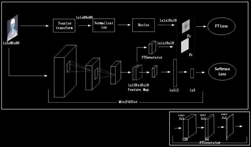
Because human skin reflects light differently than digital screens or matte paper, spoofed media reveals distinct spectral anomalies, moiré interference, and frequency cutoffs that are readily detected in the Fourier domain.
References
- A. C. Paiva (2010) — Image representation, sampling, and quantization, ECE 6962
- NV5 Geospatial Software (2026) — MEAN_FILTER, NV5 Geospatial Software: https://www.nv5geospatialsoftware.com/docs/MEAN_FILTER.html
- I. Ozhiganov (2017) — Convolutional Neural Networks vs. Cascade Classifiers for Object Detection, DZone: https://dzone.com/articles/cnn-vs-cascade-classifiers-for-object-detection
- Minivision AI (2021) — Silent-Face-Anti-Spoofing, GitHub Repository: https://github.com/minivision-ai/Silent-Face-Anti-Spoofing/